How to cheat at stats

Misapplied basic statistical tests are remarkably prevalent in the biomedical literature. Some of the most common and egregious mistakes are illustrated below. Experts in statistics will consider my explanations simplistic and marvel that people don’t understand such matters. However, perusal of the biomedical literature, including almost any issue of glamour journals like Nature or Cell, will convince you that the problem is real and that the misunderstandings are shared by editors, referees and authors. By a totally unsurprising coincidence, these errors usually have the effect of increasing and even creating statistical significance.

It should be noted that I’m no expert in statistics. Consider this a guide by a statistical dummy for statistical dummies. I have made some of the mistakes outlined below in my own research; I’m only one step ahead at best… I should also add the disclaimer that, despite its title, the purpose of this post is of course education and prevention, not as an incitement to cheat.

Use of pooled unequal variances in ANOVA post-hoc tests

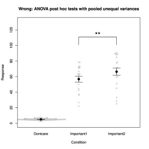
ANOVA tests are frequently used when an experiment contains more than two groups. The omnibus ANOVA test reports whether any deviation from the null hypothesis (all samples are drawn from the same distribution) is observed and then a post hoc test is almost always applied to evaluate specific differences. Standard ANOVA is a parametric test and therefore incorporates the prerequisites of randomness, independence and normality. Furthermore, and critically, it also assumes that all groups have the same variance (homoscedasticity), because the null hypothesis assumes a common distribution. When post hoc tests are applied, they generally use the pooled variance, which is the combined variance from all of the groups. Violation of the condition of equal variance opens the possibility for quite erroneous results to be obtained from the subsequent post hoc tests. It works in the way illustrated in Fig. 1. Imagine three experimental groups, of which only two rather variable ones are really of interest (labelled “Important” in the figure), while the uninteresting one (labelled “Dontcare”) has the largest sample size and a much smaller variance. If we compare the two Important groups directly using a t-test, we find they are not significantly different (p = 0.12). If we apply ANOVA despite the violated equal-variance condition, we find first that the omnibus test reports a very significant deviation from the null hypothesis (p < 10^-15). This is unsurprising, because the “Dontcare” group clearly has a different mean from the two “Important” groups. Then, the application of the post-hoc test, even with corrections for multiple comparisons (as should be), reports that the two “Important” groups differ significantly (p = 0.009). Yet the direct comparison of the same two groups, without any correction for multiple comparisons, was non-significant! We see that this significant result has been created by the use of the pooled variance in the post hoc test. That variance was artificially lowered by the invalid inclusion of a large group with a much smaller variance.

Clearly, in real life, sample variances will never be exactly equal, so what difference is acceptable? A frequent suggestion is a factor of no more than 4 in variance, so a factor of 2 in standard deviation. (Note, however, that what is often plotted is the standard error of the mean, in which case unequal error bars might also arise because of unequal sample sizes.) But why not dispense with the ANOVA entirely? There is in reality little use for the one-way ANOVA unless one is specifically interested in the omnibus test of a collective violation of the null hypothesis that all groups are sampled from the same population. Usually, one is interested in specific differences between groups, in which case it is perfectly valid to apply direct tests with correction for multiple comparisons, as long as pooled unequal variances are not used.

For direct tests that control false positives under most conditions, consider the Welch test, which is explicitly designed to work with unequal variances and is quite robust to non-normality, or the fully non-parametric Brunner-Munzel test. In contrast, and perhaps surprisingly, some of the well known rank tests like Mann-Whitney, Wilcoxon and Kruskal-Wallis are not such good options, because, although they do not require normality, they do require all groups to have the same distribution; different variances would violate that prerequisite. If the condition is not satisfied, the result must be interpreted as testing “stochastic dominance” rather than a difference of medians.

Note: it turns out that there are both ANOVA equivalents and post hoc tests suitable for groups with unequal variances, namely Welch’s ANOVA and the Games-Howell test.

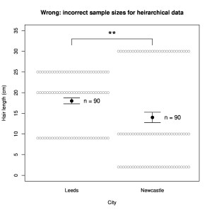
Incorrect sample sizes for hierarchical data

Imagine testing the hypothesis that people from Newcastle (“Geordies”) have different length hair than those from Leeds (I just learnt they are called “Loiners”). As often occurs in the modern literature, we only gather very small samples, n = 3 inhabitants from each city. (It is basically impossible to justify the validity of any statistical tests on such small samples. Experiments with such small samples are moreover almost always underpowered, which introduces additional problems. I use them here because they are still quite common in the publications containing the errors I am illustrating. The error mechanisms do not depend on the sample size.)

We take one hair from the head of each person and measure its length, obtaining in cm:

Newcastle: 2, 10, 30
Leeds: 9, 20, 25

Following standard procedure, we apply a (probably invalid) t-test to these samples and find that their means are not significantly different: p = 0.7. Irrespective of any true difference between the populations (in truth I expect none), the experiment was desperately underpowered because of the small samples. Unsurprisingly, therefore, no difference was detected.

Now let’s modify the experiment. Instead of measuring one hair per person, we measure 30 hairs per person. Each number above now appears 30 times (the numbers are exactly equal because the subjects all have pudding-basin cuts):

Newcastle: 2, 2, 2, … 10, 10, 10, … 30, 30, 30 …
Leeds: 9, 9, 9, … 20, 20, 20, … 25, 25, 25, …

Much bigger samples! Now if we apply the t-test with n = 90 for each sample, we obtain a difference that is satisfyingly significant: p = 0.006.

But of course this is nonsense. The example was chosen to highlight the cause of this erroneous conclusion—the samples are no longer independent. For hair length, clearly most (all in our example) of the variance is between subjects, not within subjects between hairs. In such experiments, variation between the highest-level units (here subjects) must always be evaluated. A conservative approach is simply to use their numbers for the degrees of freedom. However, further information about the sources of variance can be obtained by using more complex, hierarchical analyses such as mixed models. Note, however, that more sophisticated analysis will never enable you to avoid evaluating the variance between the highest-level units, and to do so experimentally you will nearly always have to arrange for larger samples than above.

This problem often goes by another description—that of biological and technical replicates, where one makes a distinction between repeating a measurement (technical replicates) and obtaining additional samples (biological replicates), with the latter representing the higher-level unit. The erroneous practice is also sometimes called pseudoreplication.

Applying two-way ANOVA to repeated measures

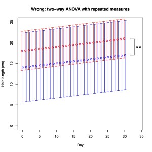
For our next trick we return to our initial samples of hair measurements. With n = 3 people per sample, there was no significant difference between Newcastle and Leeds (p = 0.7). Imagine now that we measure the length of hair of each subject every day for 30 days. We find that everybody’s hair grows 0.1 mm per day. A common error in such situations is to identify two variables (factors), in this case City and Day (time), and therefore to apply two-way ANOVA (there are two factors, right?). If we do this here, the test reports that City now has a significant effect with p = 0.006! The problem is that the two-way ANOVA assumes independence of samples, whereas we in fact resampled from the same subjects continuously. We have in effect assumed that 3 x 30 = 90 independent samples were obtained per group. Specific repeated measures tests exist for such non-independent experimental designs and they would not report City as having a significant effect in this case.

An entirely equivalent issue arises when performing any statistical inference on regression lines (or curves); it is critical to understand whether the data points are independent or not, and the correct test will almost certainly differ in consequence. xkcd has offered a similar illustration.

Failing to test differences of differences

Maybe most of us have done this one? You test an intervention in two different conditions, yielding four groups to be analysed. A recurring example is testing whether some effect depends upon the expression of a particular gene, which is investigated by knocking out the gene. Typical results might resemble those in Fig. 4. The intervention has quite a respectably significant effect (Test vs. Ctrl, p = 0.003) in the wildtype (WT), while in the knockout (KO) mouse the effect is almost absent and no longer significant at all (p = 0.6). However, inference cannot stop there. One needs to test directly whether the difference in the wildtype is different to that in the knockout. One way of doing this is to examine the interaction term of a two-way ANOVA; bootstrap techniques could alternatively be used. In fact, analysing these data with a two-way ANOVA reveals that the interaction between genotype and condition is not significant (p = 0.09).

Another way of remembering the necessity of performing this test is the following expression: “The difference between significant and non-significant is non-significant”.

A related problem arises when a two-way design like that above, which is designed to examine whether there is a non-additive effect of the “test” and “genotype” factors, is analysed as a one-way design. In such cases authors generally sprinkle a few stars on the significant differences, but none actually supports the existence of a non-additive effect.

Conclusion

ANOVA tests are surprisingly complicated. Their correct application depends upon a long list of prerequistes, with violations of independence and equal variance being particularly dangerous. Simply managing to feed one’s data into an ANOVA is not nearly enough to ensure accurate statistical evaluation. The misapplication of ANOVA tests offers numerous possibilities for overestimating the strength of statistical evidence.

If you come across examples of the misuse outlined above, why not comment them on PubPeer?

PS. It turns out that there is an excellent book that overlaps with some of the above material; it is well worth reading: Statistics done wrong. Moreover, the chapters have been made freely available online, so there is really no excuse.